GRC Transmission Analysis: Getting To the Bytes

Post Author: Don C. Weber [Twitter: @cutaway]
Date Published: 15 May 2014

I have not picked up my HackRF Jawbreaker in a while (Figure 0x0). Family and billable work trump side projects. Lucky for me Tom Liston and I started teaching the Assessing and Exploiting Control Systemsclass which leverages the Samurai Project’s Security Testing Framework for Utilities (SamuraiSTFU). I say “lucky” because I have a few updates I want to work into the courseware that center around improving the GNU Radio Companion (GRC) frequency analysis labs. Even with the SamuraiSTFU updates I still found myself busy. I kept putting this off until Jay Radcliffe asked me to take another look at a radio capture he had grabbed from his insulin monitor/pump setup. He wanted to see if we could use GRC pull the transmitted data out of the air and into a file as I had done a couple months before with RFcat.

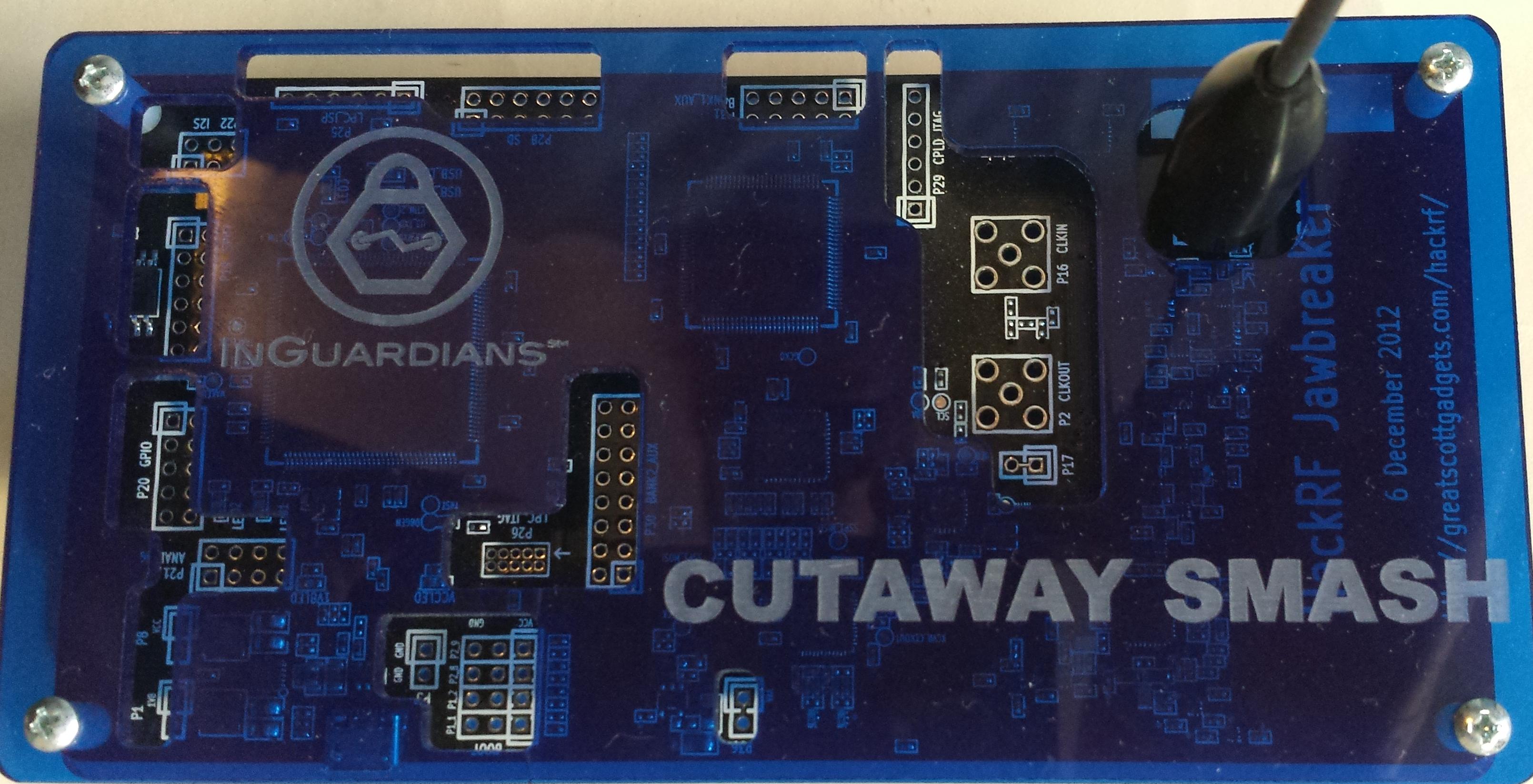
Figure 0x0: HackRF Jawbreaker

Both of these projects had a similar issue: we were having difficulty moving from the captured radio transmission to actual demodulated data representing a “packet” of bytes. There are several reasons for this predicament, but the biggest issue is the recent advances to GRC. The rapid development and growth of the GRC code over the last year has been staggering. All of my old GRC files use blocks that are listed as “Old” or the blocks that do not appear in the main GRC window at all. The most frustrating case, of course, is when the blocks don’t appear at all because I have to try to remember what I was trying to accomplish a year ago. Imagine opening up a script you wrote a year ago (one you didn’t really fully understand at the time) only to find out that fifty percent of the functions had been deleted, seemingly at random.

Another general issue related to proper signal processing is that each block has its own parameters that are specific to efficient processing of the signal into a demodulated state. For those of us who are not radio engineers and do not work with GRC every day, understanding these parameters is extremely difficult. If you don’t understand exactly what they do, how can you know how some of these parameter values are obtained or modified? Let’s face it, there is a LOT of math involved with frequency analysis and demodulation. Fortunately, tools like GRC exist to do the majority of the difficult math for us. However, many of these math functions require very specific values so that the results of the computations are accurate for the specific signals being analyzing.

Like everyone else, my family and billable work issues never let up. Thus, I found myself, as most of us do, working deep into the night on these “side projects.” Here are a few things I learned – by asking questions, reading blogs, using default settings, and (in true hacker fashion) guessing through trial-and-error.

Before we start, I have created a white paper for those people who are impatient, do not like the conversational tone of a blog post, or want to have this information in a document to read and pass around:Converting Radio Signals to Data Packets. Additionally, for quick reference, I will be using a tool called GRC Bit Converter to help analyze and print the captured data.

Managing Direct Current Spike

When using a HackRF or one of the many RTL-SDR dongles there is a large spike at the center frequency to which the radio has been tuned. This is the Direct Current (DC) spike (demonstrated using SDR# in Figure 0x1), that occurs naturally in radios that have not specifically accounted for this spike via hardware / firmware. The HackRF team does a great job explaining why this occurs and what can be done with it in their website’s Frequently Asked Questions (FAQ).

Figure 0x0: HackRF Jawbreaker’s DC Spike

As described in the HackRF FAQ, the DC spike can simply ignore it. However, because I have had a hard time successfully demodulating the signals recently, I want my data to be as clean as possible (yes, I am probably a little naive, but learning this also method helps when I “do” need it).

To avoid the DC Spike, I like to create my captures by leveraging the “DC Offset” method. Capturing with an offset is easy enough to understand and easy to accomplish with the currently available GRC blocks. The challenge here is to select an offset that moves our DC Spike outside of our source’s transmitted signal while still staying within the bandwidth that is being captured. There are two methods can be leveraged to determine this offset. The first is to conduct data sheet analysis to determine the radio and devices capabilities. These documents will outline “Channel Spacing.” The channel spacing is the distance between the center frequencies of two transmission areas configurable by the radio. While this helps, and is often enough information to adjust for the DC Spike, the channel spacing is not necessarily related to the size of the transmission. We see this in Wi-Fi which has fourteen (14) channels but the transmission of a wireless adapter will engulf approximately six (6) of those channels. To compensate for this possibility I use spectrum analysis software, as shown in Figure 0x2.

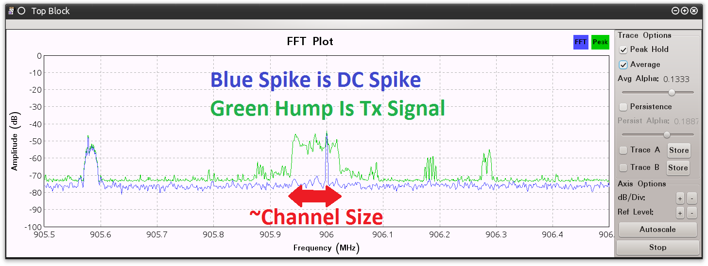
Figure 0x2: DC Spike Inside TX Signal

The spectrum analyzer allows me to visually select a frequency in an area outside the transmission. Once I have selected a frequency, I note the distance between them and configure my GRC variable blocks appropriately. In this example I will add a variable block named “channel_spacing.” This allows me to configure the Frequency Offset in another variable block, named “freq_offset”, with the equation: “(channel_spacing / 2) * (channel_spacing * .1)“. Dividing the channel spacing by two gives me the distance from the center frequency to the edge of the transmission. Using this number should move the DC Spike to the very edge of the transmission. Adding an additional 10 percent to this offset “should” move it completely outside the transmission. Figure 0x3 demonstrates the “freq_offset” variable block configuration and Figure 0x4 shows how it is implemented within the source block.

Figure 0x3: GRC “freq_offset” Variable Block Configuration

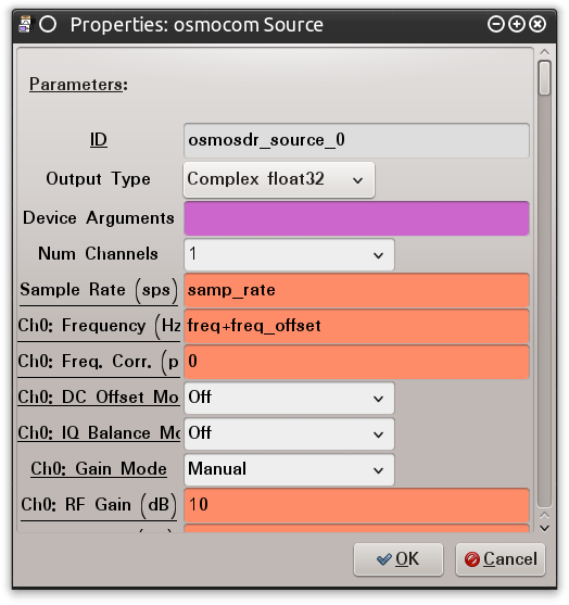
Figure 0x4: GRC “osmocom Source” Block Configuration

Once this is all configured, each of the blocks in the primary GRC window will display the computed values after doing the math for us. Each of these values is shown in Figure 0x5.

Figure 0x5: GRC Capture Configuration

When this GRC script is run the Top Block will display the location of DC spike in relation to the transmitted signal. Figure 0x6 shows how this will appear in a spectrum analyzer.

Figure 0x6: GRC Top Block With Offset DC Spike

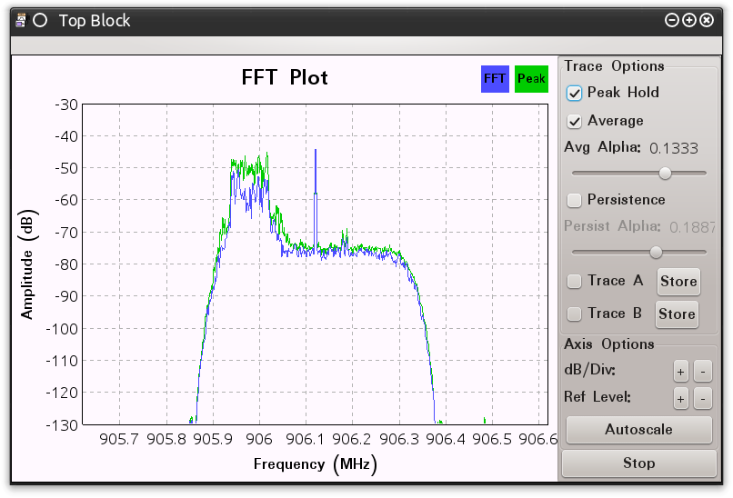
Figure 0x7: GRC Top Block Using Low Pass Filter

[Dramatic Pause] <- cause I don’t know any other way to dramatically pause in a blog post.

Look good?

[Dramatic Pause] <- /me sips a beverage

Okay, I’m just going to say it. The signal in Figure 8 IS isolated. However, it is not located at the center of the FFT Plot. If we don’t address this it will negatively impact the rest of our demodulation efforts. We need that signal centered. Right now it is centered on our DC Spike because we configured our radio to listen just outside of the transmission. Can we do it? Of course we can. We can leverage mathematics and configure a bunch of blocks to modify the output of the LPF block to compensate for our output. Or….we can use the “Frequency Xlating FIR Filter” (FXFF) block instead.

Stay with me, don’t get angry. I needed to describe the LPF because in some instances you might need to use that block instead of the FXFF block. Also, the core variables that configure the LPF also properly configure the FXFF block. The FXFF has “Decimation” and “Sample Rate” like the LFP and they are configured the same way. The FXFF block also leverages the “Center Frequency” variable. This is the variable that re-centers the signal as adjusted for the DC Offset (in other words, if you didn’t adjust to shift the DC Spike, this parameter should be left as zero (0)). What is left is the “Taps” parameter. I have no good explanation for the “Taps” parameter. However, learning from Dragorn’s blog posts “Playing with theHackRF – Keyfobs” I can see that it is related to accounting for the “Window,” “Channel Width,” and “Transition Width.” Therefore I configure the Taps value, as shown in Figure 0x8, with the following equation: “firdes.low_pass(1, samp_rate, channel_spacing, channel_trans, firdes.WIN_BLACKMAN, 6.76).” Basically, the LPF wrapped up into one variable.

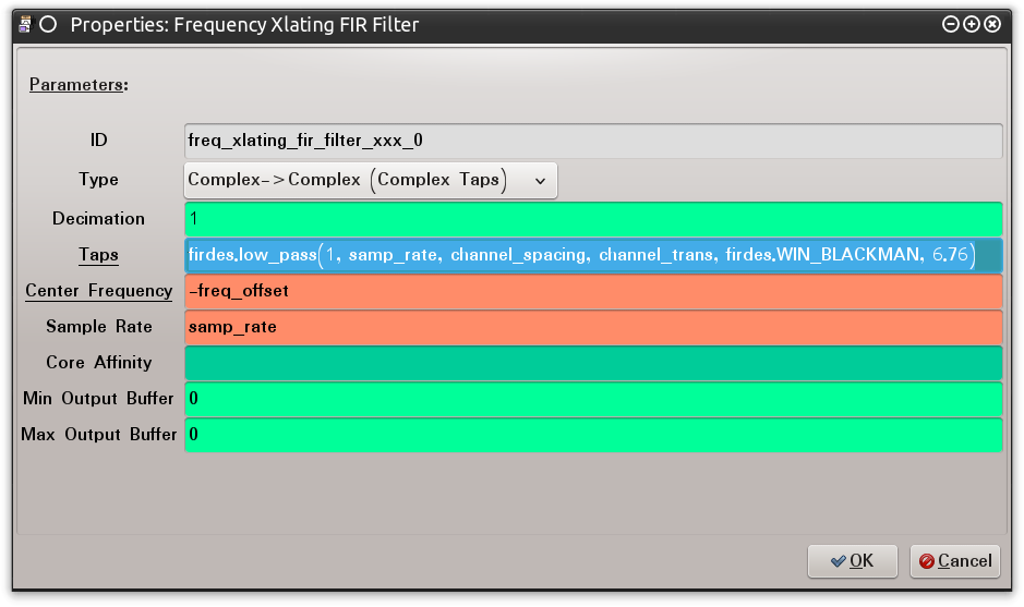
Figure 0x8: GRC FXFF Block Configuration

Running with this configuration we see, in Figure 0x9, that we have a transmission signal that is centered and ready for demodulation.

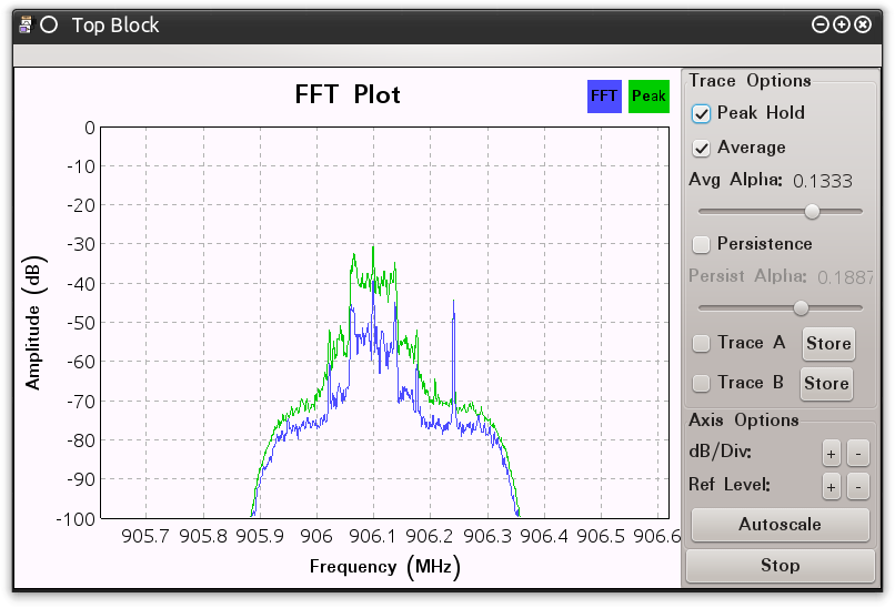
Figure 0x9: GRC Top Block Using FXFF Block

Actual Demodulation

Now that I have asignal isolated, I can start working with it. This, for me, is also the area where it starts to get a little fuzzy on “why” we perform particular steps. I’ll briefly describe what I know, but I recommend that you watch for Mike Ossmann to post his radio classes (a by-product of his successful HackRF Kickstarter project). They should provide you with the specific mathematical reasoning behind each of the blocks necessary for demodulation – both for frequency-shift keying (FSK) and for amplitude-shift key (ASK) modulation. The basics are this: the “Complex to Mag” or “Complex to Mag ^ 2” blocks are used to demodulate ASK transmissions and the “Quadrature Demod” block is used to demodulate FSK transmissions (specifically 2FSK and GFSK).

The signals I am capturing for this example leverage GFSK modulation. This, however, begs the question: “How do you know this?” Plainly, I know the device that is transmitting and capturing the transmissions.

What we are seeing in the previous images is the results of a Texas Instrument (TI) Chronos Watch communicating with the TI Chronos Dongle. The TI Chronos Dongle has a TI Chipcon CC1111 radio. The datasheet and even the source code for the dongle are available on TI’s website. Often times, a radio’s datasheet is sufficient to provide all of the information needed for demodulation. Having source code, however, is always better – because nearly every radio can be configured in a wide variety of ways. A vendor will configure the radios in their products to perform optimally for the device’s primary functionality. Datasheets narrow the possibilities, while source code and radio configuration settings provide specifics. In the case of the TI Chronos Dongle, doing a quick review of the source code, provides the values used to configure the radio for interaction with the TI Chronos Watch (see Figure 0xa).

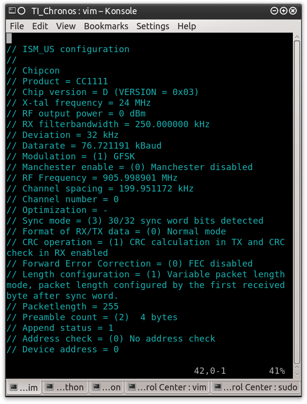
Figure 0xa: TI Chronos Dongle Source Code Radio Configuration Settings

Reviewing these settings, you will notice some of the parameter values that have been used to configure the previous block variables. Remember these settings – we will be coming back to this for additional parameter values as we progress. To continue on the “path to demodulation” I am most interested in two of these values: the modulation type and the “Deviation”. The modulation, as mentioned before, is GFSK and therefore requires that we use the “Quadrature Demod” block for demodulation. This block needs to be configured with the Deviation value.

The actual parameter that needs to be updated is the “Gain” value. The Gain parameter is preconfigured with the following equation: “samp_rate/(2*math.pi*fsk_deviation_hz/8.0)“. To complete this we just need to create a “fsk_deviation_hz” variable block with the value “32000” as defined by the Deviation value in the source code. While I am at it, I usually also define a “data_rate” variable and update the “freq” variable to be more precise. Figure 0xb shows these modifications with the addition of the “Quadrature Demod” and “fsk_deviation_hz” variable blocks.

Figure 0xb: GRC Quadrature Demod Configuration

As Figure 12 shows, the “Quadrature Demod” block has been configured to to output to a “File Sink” block. I could have also output to another “FFT” block but the active demodulation will not be very interesting other than showing it is working. To actually “see” interesting demodulated signal it will take other wave analysis tools. But before we do, I should explain several things that need to be taken into consideration. The first is that capture files from radio transmissions can get very large, very fast. Capturing straight from the HackRF to a file with a sample rate of 1,000,000 will generate approximately one gigabyte every forty (40) seconds, and data size increases dramatically as you increase the sampling rate. For these instances you need to consider if your analysis machine is capable of writing to a hard drive fast enough to keep up with the data being captured. Often, if I am capturing straight to a file I will output to the “/dev/shm” directory which is provided by my Linux-based operating system. This is RAM Disk and it can be written faster than a hard drive (system dependent, of course). When post-processing a previously saved capture to demodulate the data, however, we don’t need to worry too much about write speeds as long as we’re careful to monitor file sizes so the hard drive does not become filled.

One side note: It is extremely importing to remember – for all capture files – information about our capture settings. Without knowing these settings, we will not know how to analyze or replay the data in the future. To address this, I always note all of the settings that are important for analysis in the capture file name. In this case I will be using the filename: “/tmp/blog_demod_1e6_905.99e6_gfsk_76721_hackrf.cfile” I’ll let you match these values to their appropriate configuration settings.

Hitting the run button will initiate the radio capture, and the transmission will be processed through the demodulator and output to a file. As it was the tool I was trained on I prefer viewing the resulting signal using Baudline. I could explain exactly how to pull the demodulated file into this tool but this has already been explained very well by Dragorn in his Keyfob blog post. Rather I am going to show, in Figure 0xc, the captured demodulated signal as seen in Baudline using the primary FFT and the Waveform display.

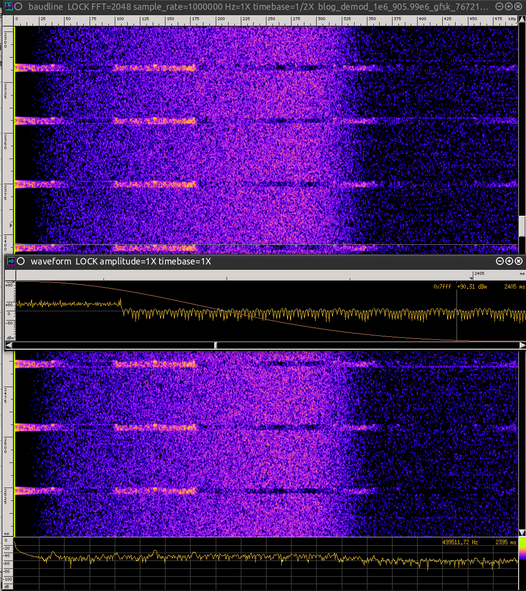
Figure 0xc: Demodulated Capture Displayed in Baudline

The signal displayed in the center window, the “Waveform” display, is what we are most interested in. The FFT that you’re seeing behind it is actually a waterfall display that shows the demodulated signal over time where the data is “generally” represented by clumps of noise. The Waveform display shows the demodulated signal at a particular moment in time in relation to the primary FFT. Using Baudline in this manner allows me to analyze how the signal looks before it is passed onto the other GRC blocks that will be used to determine the actual “ones and zeros.” That’s right –at this point the wave shown in the Waveform display should be the transmission’s data. Figure 0xd is a closer look at this wave.

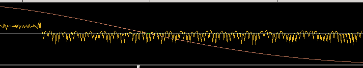
Figure 0xd: Demodulate Capture Displayed in Waveform Display

Reviewing this image using my training and experience I can tell three things:

1. This signal is not clean enough. It does not appear to be a nicely formed wave with smooth transitions.
2. The wave is actually shifted slightly and does not cross the center-line optimally.
3. In order for the data to be processed in GRC and properly convert to 0’s and 1’s the wave will have to be “cleaned up.”

Hardware radios actually do this “cleaning” process using the circuitry designed into the radio component. Radios implement a LPF after the demodulation before converting the transmission into data.

Therefore, to properly process this transmission I need to implement a LPF in the GRC script.

This part may generate a bit of confusion. Because I have no good explanation for the values that I select when creating the LPF that follows a demodulation block – it really is a trial-and-error process that I keep “tweaking” until the data “looks right.”

From the earlier explanation of the LPF parameters the “Cutoff Freq” and “Transition Width” parameters (“Window” should be updated to “Blackman”) will need to be configured. For the “Cutoff Freq” I usually start with a value of 100,000 and then select a “Transition Width” about half of that value. Once configured, I capture the transmission again, or replay a previously captured transmission, to process it through the demodulator. I do this several times pulling the results into Baudline each time, reviewing the resulting signal, modifying the values, and then capturing again. This is repeated until I see a wave pattern with nice transitions that look like data. What does data look like? Figure 0xe shows this state which was accomplished by using 80,000 for the “Cutoff Freq” and 50,000 for the “Transition Width.”

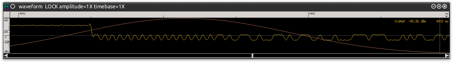
Figure 0xe: Demodulated Signal Run Through a LPF

Taking a closer look at this signal I can see that it is not centered on the X-axis. A good wave pattern, that is ready for processing by the next GRC blocks, will be centered. This may merely be a visual pet peeve of mine, but in my experience the following blocks successfully output the data when the wave is centered on the X-axis. Shifting this wave up (or down if need be) is simple by using mathematics. If I were to multiply each point on that wave by a number it will increase the amplitude of the wave pattern. In this case I don’t need to increase the amplitude. I need to move each value “up” on within this display. Thus, instead of multiplying each point I add a constant value to each point. The increased value of the point is represented on the Y-axis and thereby shifts the wave up. In contrast, I can subtract a constant value from each point to shift it down. The actual value is determined via experimentation and observation and implemented using the “Add Constant” block. The results of shifting this wave pattern by adding a constant value of 6 is shown in Figure 0xf.

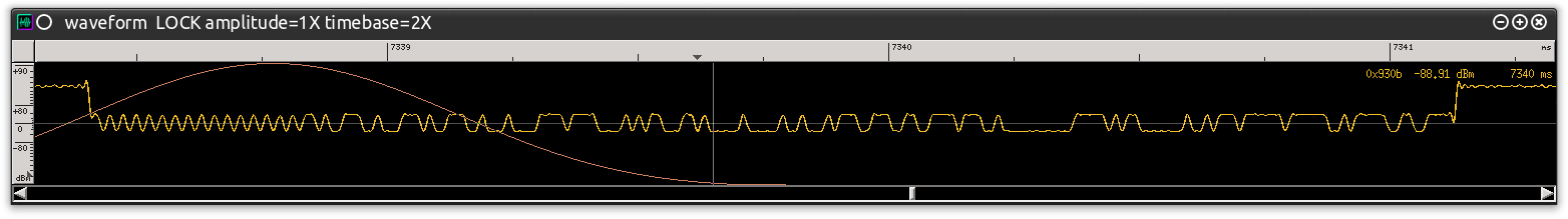
Figure 0xf: Demodulated Signal Shifted Up to X-axis

 

As I mentioned, I am not sure how important that last shifting step is in this whole process. But knowing “how” to manipulate the wave pattern without losing any data could help us in the future. For instance, if you know the data is being transmitted inverted (meaning a 0 is a 1 and a 1 is a zero) how could you manage it with these tools? Would multiplying by a negative constant help? Try it out.

Counting the Bits

Now that I have a nice clean demodulated signal I can move onto the next step. This step involves taking this wave signal, analyzing the highs and lows for a logical pattern, and then using that information to discern 0’s from 1’s. It is all in the mathematics, and GRC has it figured out for me. I start with two specific blocks: “Clock Recovery MM” and “Binary Slicer”. The “Clock Recovery MM” block does the magic of discerning highs and lows. The “Binary Slicer” marks the highs as a “1” and the lows as a “0”. Actually, it marks them as “0x00” or “0x01” which I will need to manage, later. For this all to work I need to concentrate on configuring the “Clock Recovery MM” block correctly.

The “Clock Recovery MM,” shown in Figure 0x10, has some REALLY scary looking parameters (cause math is hard). Fortunately, I took Mike Ossmann’s training course and I don’t worry too much about them – they’re actually fairly easy. When I drop the block into the GRC script, it is set with a bunch of default settings for its parameters. As per Mike, do not touch “Gain Omega,” “Mu,” “Gain Mu,” or “Omega Relative Limit” – leave them as the default values. I’ve never changed them and I have always been told to leave them alone. Someday I may learn a need to modify them – but not today. Today I only need to concentrate on the “Omega” parameter. This parameter also comes set to a default value: “samp_per_sym*(1+0.0)“. Oh, look, a variable name. Looks like it wants me to set up a variable block with the name “samp_per_sym” which equates to “Samples Per Symbol.”

Figure 0x10: GRC Clock Recovery MM Block Configuration

I do not have the actual value for “Samples Per Symbol,” yet. But I do have the values necessary to compute this value. The value for “samp_rate” is actually “Samples per Second”. For this capture that is 1,000,000 samples per second. The “Data Rate” from the radio configuration file is actually “Symbols Per Second.” I have already added this as the “data_rate” variable with the value: 76721.191. Simple mathematics helps me create a “Samples Per Symbol” parameter by dividing the “Samples Per Second” parameter by the “Symbols Per Second” parameter. The “Per Second” values will cancel each other out and I am be left with “1,000,000 / 76721.191” which is the value for “samples per symbol.” Creating a “samp_per_sym” variable block with the entry “int(samp_rate / data_rate)” is what I want to do and is shown in Figure 0x11. This will automatically calculate the “Samples Per Symbol” and make it an integer for the “Clock Recover MM” block.

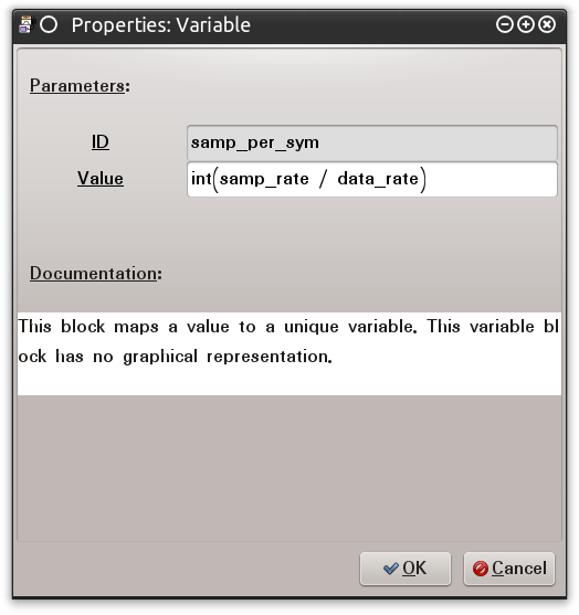
Figure 0x11: GRC “samp_per_sym” Variable Block

With the variables for the “Clock Recovery MM” block configured we can have it identify the 0’s and 1’s for us. But we need a place for these to go. Therefore, another “File Sink” block is in order. I usually just write this to the “/tmp” directory and give it an extension of “.dat”. Figure 0x12 shows the current GRC setup.

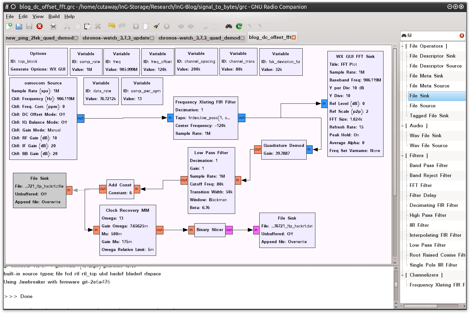
Figure 0x12: GRC with Clock Recovery MM To Extract Data

 

Analyzing Demodulated Data

Running with the “Clock Recovery MM” and “Binary Slicer” blocks will provide me the demodulated data I want. Figure 0x13 shows how this data looks when I review the contents of the output file using the “xxd” command.

Figure 0x13: Demodulated Data Viewed Using “xxd”

 

As mentioned, it is a file full of 0’s and 1’s, literally. What I need to do now is basically squash each one of those lines into a byte. The first line “0101 0101 0101 0101 0101 0101 0101 0101” actually translates to “0b1111111111111111” or “0xff”. The line starting at offset 0x30 is “0101 0101 0101 0101 0001 0100 0100 0101” or “0b1111111101101011” or “0xff6b”.

This output looks very promising, but anything can spit out 0’s and 1’s. How do I know if this is actually the data I want? Excellent point, and I will tell you that what you see in Figure 20 is very possibly just noise floating through the air.

You see, the “Clock Recovery MM” block did exactly what I told it to do. It looked at the incoming signal, made an estimation as to whether that signal was high or low, passed it to the “Binary Slicer” which converted “High” and “Low” into “1” and “0”. However, as with anything, there is a lot more noise out there than there is actual signal. I have not told any GRC block how it can tell the difference between the signal I want, the signal from another radio, or just noise in the air. Also, even if a block does understand that it is receiving actual data, which bit is that bit in the byte? The Most Significant Bit? The third bit from the Least Significant Bit? Always remember – in radio, the data receive is just raw data… it could be anything from the data I want to noisy garbage. I need to take a long, hard look at the raw data output by GRC and the “Clock Recover MM” to see if I can make sense of it.

Luckily, we are programmers at heart, right? Well, I am a scripter anyway. It might take a little while, but anybody who has made it this far into this blog post will probably know how to take a file, grab each raw “data” byte, and squash it into a “real” data byte. For those of you who cannot, or do not have the time, I have written “grc_bit_converter.py” as seen in Figure 0x14.

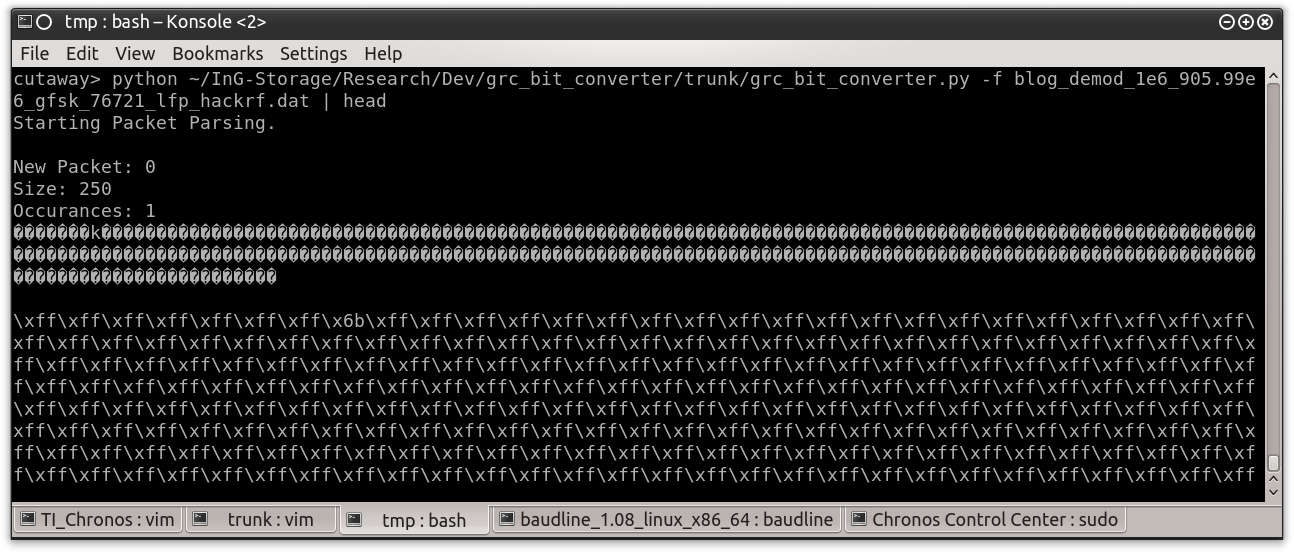
Figure 0x14: Processing Radio Data using “bit_convert.py”

The “grc_bit_converter.py” script allows me to process the data output created by the “Clock Recovery MM” block in several ways. If I run the tool with the default settings it will start at the beginning of the file, pull out the first 250 bytes, and prints the results in “raw data” and “data byte” format. The script considers these 250 bytes to be a packet and continues to process all packets until the end of the file. Each of these packets is marked with a packet number for easy identification. The “Occurrences” value shows how many packets contained the exact same data which will be very useful once we find actual transmissions. Of course the packet size variable is configurable, but for now I will leave this setting with the default value.

Now that I have pulled some “data” from the transmission I need to think about how that data will be formatted so that I can search through the converted information. Most radios (not all, but most) will begin a transmission with some type of “preamble” followed by a SyncWord. Preambles are generally a series of high to low transitions. When viewed in binary these will appear as “0b1010101010101010” or “0xaaaa”. The number of preamble bytes depends on the radio and how it is configured. As the tool does not know exactly which bit is the first bit (or if the transmitted data has been inverted) the preamble may appear as “0b0101010101010101” or “0x5555”. The job of a preamble is to let the radio know that incoming data is on the way and that it that should get ready to process it. The job of a SyncWord is to tell the radio where the actual data packet begins. It can also be used as a designator between two different networks. Any value can be picked for the SyncWord with the obvious exceptions being those that closely resemble a preamble. The most common that I have come across is “0xd391” (look back at Figure 16 and see if you can find this value in the waveform). Like the preamble I need to think about how this might appear in a data file. I can easily do this using iPython and shifting the bits to the left one bit at a time. Figure 0x15 shows that if the sync word is “0xd391” it may actually appear as “0xa722”, “0x4e44”, or “0x9c88” when I am reviewing the bits of a data transmission.

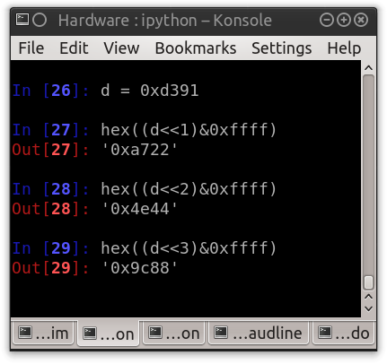
Figure 0x15: SyncWord Shifted By One, Two, and Three Bits

 

With this knowledge I can now search the parsed data for transmitted data packets. For this exercise I have decided to just output the converted data to “less” and then search for the known SyncWord “0xd391” using “d3\\x91”. Figure 0x16 shows the results of this search and one of the transmitted packets.

Figure 0x16: SyncWord Search In Data Output by “grc_bit_conveter.py”

To me, this definitely looks like a data packet. I can confirm this with collaborating information by looking back at the source code for the TI Chronos Dongle. The source code specifically states that the Preamble count is two (2) which is equal to four (4) bytes. The Preamble of this packet is “\xaa\xaa\xaa\xaa” which is also four (4) bytes. It states that the Sync mode is configured to detect 30 bits of a 32 bit sync word. The SyncWord of this packet is “\xd3\x91\xd3\x91” which is 32 bits. It states that the packet length is variable and defined by the first byte after the SyncWord. The first byte after the SyncWord is “\x0f” which equates to fifteen (15). From the end of the length byte I can count out fifteen bytes and I are left with two bytes before the bit stream reverts to all 1’s or 0xff. These last two bytes are the Cyclic Redundancy Check (CRC) for the packet which, according to the source code, has been enabled.

Marking The Packet

Finally, I have a packet of data. I can output this data to a file, go through it and manually or with a script to pull out the data of interest, and begin my analysis. When information is limited this is exactly what I will do. But in this case I have a lot of information about the transmission. Heck, even with just this raw data I should be able to make some logical assumptions to perform the next steps: marking the data packet when it is captured using GRC. If I do it correctly the data in our output file will be marked exactly where packets begin.

Marking packets in GRC is accomplished using the “Correlate Access Code” block. This block will take two values: “Access Code” and “Threshold”. The Access Code is a sequence of bits (0’s and 1’s) that indicates the beginning of a packet. This block will use this value and monitor the data passing out of the “Binary Slicer” block. If it sees this sequence of bits in the byte stream it will mark the next bit it processes by flipping the second bit of the byte. Remember, the information coming out of the “Binary Slicer” is a full byte of data for each 0 and 1 in the binary data stream. By flipping the second bit of this byte the byte is converted from a “0” or “1” to a “2” or “3,” respectively. This data can still be analyzed and converted as the Least Significant Bit is not modified. The “Threshold” variable merely indicates the number of bits that can be “different” than the actual value provided in the “Access Code”. This is done in case an incoming packet is slightly corrupted but can still be processed. It allows the radio to leverage other means to manage transmission errors. Figure 0x17 shows the “Correlate Access Code” configured with the “0xd391d391” bit sequence and a “Threshold” of two (2) as indicated in the source code. Had I not known the SyncWord I could have used the binary value for the Preamble.

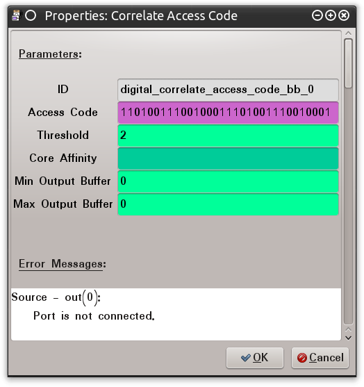
Figure 0x17: Correlate Access Code Configured with 0xd391d391

As mentioned, the “Correlate Access Code” block processed the data exiting the “Binary Slicer” block. Figure 0x18 shows the placement of these blocks so that the output it directed into a data file.

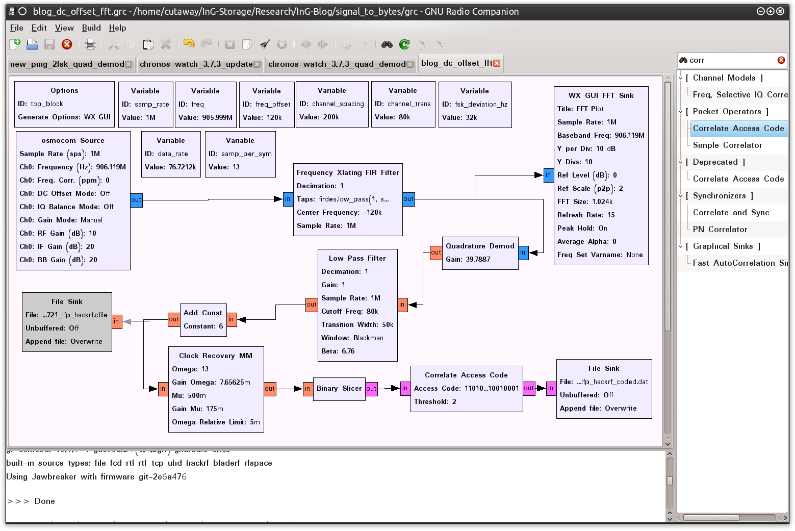
Figure 0x18: GRC Configured with the Correlate Access Code Block

After capturing the transmissions with this GRC configuration I can analyze the data as I did before. Starting with a quick review using “xxd” I can search for a value of 02 or 03 to see if I have any marked packets. Figure 0x19 shows one of these packets.

Figure 0x19: Marked Packet Viewed Using “xxd”

Now that I have marked packets I know it is worth processing the data. As before I will use “grc_bit_converter.py” because this script has an option to detect the packet markers provided by the “Correlate Access Code” block. It also has the ability to modify the size of the packet printed to the screen. Figure 0x20 shows the first packet detected using these markers and printing a packet size of 18 which includes the length byte and the CRC. Reviewing this output quickly, I can see that it matches the criteria that I found in the previous analysis of these packets.

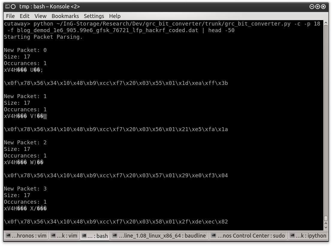
Figure 0x20: Marked Data Output by “grc_bit_conveter.py”

 

Testing The Control

Excellent, now I have packets for processing. With a little more time and effort I could take what I have here, strip out the GRC GUI components, and start building a Software Define Radio script to check, display, an interact with packets. This GRC configuration will work for the TI Chronos Watch, but will it work for other, similar, devices as well. Basically, the TI Chronos Watch is the control. Now I need a test subject. Fortunately I have been provided one by Jay Radcliffe’s question to the GNU-Radio discussion list. I worked with Jay and he provided me with a slightly different capture using the DC Offset method.

To get rolling with a transmission capture file I merely added a “File Source” and “Throttle” block. These blocks read the data from a file and throttle the data as it is passed to the rest of the GRC blocks. Throttling is performed so that the following blocks see the data at the captured rate, rather than just a straight data dump that would over-load the program. In this case the capture rate is 500,000 samples per second and the DC Offset is 200,000 Hz. The signal is being transmitted on 903 MHz using GFSK modulation. Figure 0x21 shows this capture from which I will try and determine the Channel Width.

Figure 0x21: Transmission on 903 MHz Captured with .2 MHz Offset

 

The captured transmission is close to the left-edge of the maximum capturing bandwidth as defined by the sampling rate. Although close it does look like Jay captured the full channel width. But, because it is right on the edge, I do have to be careful with my configuration settings for “Channel Spacing” and “Channel Transition” so that I do not specify an area outside of the captured bandwidth (I’m not sure how GRC will handle it if I did). Using the Frequency scale it looks like the “Channel Spacing” goes from 902,950,000 to 903,100,000 Hz giving me a 150,000 Hz channel width. Staying inside this range we will set the “Channel Spacing” to 100,000 and the “Channel Transition” to 50,000. These values are used to update the FXFF parameters. The results of this configuration update can be seen in Figure 0x22.

 

Figure 0x22: Transmission Filtered Using FXFF Block

From Jay’s GNU Radio posting I know that the Deviation for this transmission is 16,500 Hz and the data rate is 19,200 Symbols Per Second. The Deviation value is used to update the “fsk_deviation_hz” block. Once this block is configured configured I can pass the filtered data through the “Quadrature Demod” block and start my analysis of the demodulated signal using Baudline. From this analysis (and trying a bunch of different values until it worked) I got the “CutOff Freq” and “Transition Width” values for the “Low Pass Filter” block I will use after the “Quadrature Demod” block. These values are 25,000 and 10,000 respectively (this is a huge difference from the previous settings for a very similar radio and I do not know why, but it works). Figure 0x23 shows the resulting wave pattern as displayed in Baudline.

Figure 0x23: Demodulated Signal From Captured Transmission

From this image the wave form appears to need to be shifted down slightly. I ran a quick test of the data output before and after shifting this wave form and output data did appear to be different. Next, the “Add Constant” block was configured with a constant value of negative six (-6) to shift the wave pattern down. Visual review of Figure 0x23 determined that this transmission only sends the SyncWord once. Therefore I modified the “Correlate Access Code” so that it marked a packet every time that it found the SyncWord “0xd391”. This data was output to a file and the “grc_bit_converter.py” script was used to check for marked packets. Review of this data showed that some packets appear to have a consistent length of eighty (80) bytes. Figure 0x24 shows some of the packets output by the script.

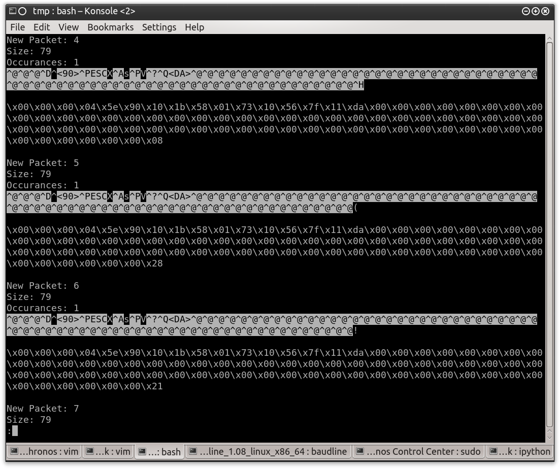
Figure 0x24: iMarked Packets Displayed using “grc_bit_converter.py”

 

Conclusion

Capturing transmissions with GRC is fairly easy once you have the proper equipment and the software installed. Understanding how to manipulate the transmissions captured using GRC is a bit more difficult. Demodulating the transmissions down to the actual data being transmitted is even more difficult. Notice, however, that I did not say “impossible.” There is plenty of information out there for conducting signal analysis. Some of this information is difficult to understand and much of it glosses over most of the important techniques and configuration settings. The information out there is extremely helpful but it only contains pieces of the puzzle. The great thing, however, is that the radio hacking community is growing very rapidly. Unfortunately not all of these people are talking, yet. Hopefully we will see more examples and tutorials soon. I am also hoping that this blog post helped fill some of the gaps and will, in turn, inspire others to do the same.

If you are looking for training on radio analysis then I highly recommend you watch Mike Ossmann and his HackRF project. Mike usually gives one or two classes a year and they contain a more in-depth understanding of radio transmissions. Everything I have provided in this blog post was born of that training and my experiences that have resulted from it.

As I mentioned at the beginning, Tom and I are teaching the “Assessing and Exploiting Control Systems with SamuraiSTFU” when Justin Searle is swamped or just needs a break. You can check out the SamuraiSTFU website for training dates and you will most likely see me in Houston and Amsterdam soon. I will be working all of this material into the course to augment what is already there. This will allow students to do everything we have outlined here with their own TI Chronos Watch setup provided by the classes hardware kit.

Acknowledgements

InGuardians – for helping me through this post and countless other things
Mike Ossmann – for being a leader, innovator, and teacher
Justin Searle – for trusting me and pushing me into new areas
atlas – for being a mentor and a peer
Jean-Michel Picod – for helping me get my GRC legs back under me

Go forth and do good things.